Documentation
Overview
Origins and design
The PhyloJunction project was born from our need to simulate arbitrarily complex SSE processes, but not being able to do so with many existing applications. A series of related diversification models had been implemented in excellent computational methods, but each of those tools made unique modeling assumptions that we wanted to relax.
Instead of reverse-engineering and modifying code written by others, however, it seemed like the path of least resistance was to write our own simulator. We also realized that our program could potentially come in handy in multiple projects, current and future, though only if written as more than a “one-off” chunk of code.
Ideally, PhyloJunction would have to be “modular” in its architecture, both in terms of its codebase as well as how models should be represented and specified. This modularity would allow future models to be more easily implemented – potentially by other developers – and seamlessly patched into PhyloJunction.
With the above in mind, we reasoned our work would be more likely to bear fruits (and faster) if we used a programming language that:
was easy to prototype and debug model code in, and
cross-platform,
supported object-oriented programming, and for which
biology and data-science libraries were available.
Python was our language of choice. As for item (4), for example, we could make heavy use of the great Dendropy library, maintained by Jeet Sukumaran and collaborators.
Modularity was achieved by building PhyloJunction around a graphical modeling architecture. This design (used in the past, see below) would not only make PhyloJunction a more flexible simulator, but also more generally useful in the future, as a tool for method development and inference.
Graphical models
PhyloJunction follows the graphical model paradigm popularized in the last decade by programs like RevBayes, BEAST and BEAST 2. In what follows, we shall offer just a brief refresher on what probabilistic graphical models are, and one simple example of their use in evolutionary modeling. Those interested in a more detailed exposition will find it in Höhna et al. (2014) and references therein (also, take a look here).
Just as with the RevBayes and BEAST programs, specifying a model in PhyloJunction amounts to writing down any number of conditional dependencies among random variables. When looked at collectively, random variables comprise a type of probabilistic graphical model called a Bayesian network. As the name suggest, such models can be described as graphs – directed acyclic graphs (DAG), more specifically – where each node (or vertex) represents a random variable, and each edge a conditional dependency between the two nodes (variables) it connects.
A Bayesian network representing a very simple model can be seen in figure 1a:
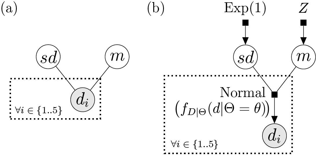
Figure 1. A simple probabilistic model represented by (a) a Bayesian network, and (b) a factor graph. From the notation in the main text, \(\theta=\{sd, m\}\). The dashed box is called a “plate”, and for each node it envelops it denotes multiple (in this case, precisely five) i.i.d. random variables. White and gray nodes denote random variables whose values we do (i.e., data) and do not know (i.e., parameters), respectively.
If we were to pen down what this Bayesian network represents in probability terms, we would arrive at a joint density (assuming continuous variables) given by expression:
where \(\theta=\{sd, m\}\).
By comparing the Bayesian network graph and the expression above, the attentive reader will notice that functions are not represented in the graph. We do not know exactly how random variables are related, other than \(d_1\) through \(d_5\) depending somehow on \(sd\) and \(m\). This is why it can be helpful to adopt a more general graphical representation: a factor graph (Fig. 1b).
The model underlying the factor graph in figure 1b is the same as that shown by the Bayesian network, the main difference being the additional factor nodes (the filled squares). Factor nodes can make the relationships between two or more random variables more explicit, especially if their (factor) functions are annotated.
In the example above we can see a factor whose function \(f_{D|\Theta}(d|\Theta=\theta)\) gives us the probability of \(\boldsymbol{d} = \{d_i: 1 \leq i \leq n\}\) given \(\theta\). It is annotated as “Normal”, so we in fact know a close-form expression for this factor function; it is the probability density function of a normal distribution. Random variables \(sd\) and \(m\) stand for the standard deviation and the mean of that normal distribution. (For those curious to see just how complicated factor graphs can be, an example can be found in Zhang et al., 2023; see their Supplementary Fig. X.)
How to read a DAG?
Most biologists specifying a DAG on a computer do so as the first step of statistical inference. They are interested in estimating unknown quantities about the natural world. These quantities – the random variables! – whose values we do not know (but would like to estimate) are referred to as the parameters of the model. Of course, parameter estimation requires that we know the value(s) of one or more random variables, which we naturally refer to as data.
In the example in figure 1, the parameters are \(sd\) and \(m\), jointly referred to as \(\theta\); the data is node labeled \(d_i\). (Note how they are colored differently, gray for data, white for parameter.) Carrying out statistical inference thus implies reading the DAG from its data nodes, normally at the bottom, towards the parameter nodes above.
The most natural approach to parameter estimation requires that we simply take the middle and right-hand side terms in equation (1), and solve for \(f_{\Theta|D}(\theta|D=d)\), the posterior density function:
This expression is known as Bayes theorem. What programs like RevBayes, BEAST and BEAST 2 do is evaluate the posterior density function at several values of \(\theta\), and output the resulting (posterior) distribution.
PhyloJunction, however, is among other things a collection of simulation (rather than estimation) engines. Borrowing the jargon used above, we are primarily interested in generating values for random variables, some of which are parameters, some data.
Here, it makes sense to think of factors as the distributions from which values will be sampled (though as we will see below, factors can also represent deterministic functions). As opposed to estimation, simulation starts at the top (or “outer”) layers of the DAG, from parameters whose values we do know, and flows in the direction pointed to by arrows (normally downwards; Fig. 1b).
In figure 1b, for example, we start from known values for the parameters of the distributions at the top. The exponential distribution from which we sample (i.e., simulate) \(sd\) has a rate of 1.0; the standard normal distribution (\(Z\)) from which we sample \(m\), by definition, has a mean of 0.0 and a standard deviation of 1.0. We then define a normal distribution from the sampled values of \(sd\) and \(m\), and in turn sample five times from that normal distribution, obtaining our data values in \(\boldsymbol{d}\).
Specifying a model (an example)
PhyloJunction takes a model specification approach that sits between those adopted by the BEAST and RevBayes communities, and that largely intersects with the LinguaPhylo project. DAG-building instructions in PhyloJunction are written in its own programming language, phylojunction (written in lowercase), whose syntax evokes RevBayes’ Rev language. But unlike Rev, phylojunction is not a fully fledged scripting language; it is lightweight and behaves more like a markup language such as XML, BEAST’s format of choice.
Commands in phylojunction can be read as mathematical statements, and are naturally interpreted as instructions for building a node in a DAG. Here is what a series of those commands would look like if written as a phylojunction script:
# hyperprior
m <- 0.0 # mean of log-normal below
sd <- 0.1 # standard deviation of log-normal below

# rate values
d <- 1.0 # death
b ~ lognormal(mean=m, sd=sd) # birth

# deterministic rate containers
dr := sse_rate(name="death_rate", value=d, event="extinction")
br := sse_rate(name="birth_rate", value=b, event="speciation")

O <- 2.0 # origin age

# deterministic parameter stash
s := sse_stash(flat_rate_mat=[dr, br], n_states=1, n_epochs=1) # parameter stash

# phylogenetic tree
T ~ discrete_sse(stash=s, stop="age", stop_value=O, origin="true")
Each line in the above script is a command instructing the application engine to take some form of user input, produce some value from it, and then store that value permanently in a new variable created on the spot.
Every command string consists of an assignment operator (e.g., <-, :=, ~) placed between the variable being created (on its left side) and some user input (on its right side).
We can look at some of these commands individually:
d <- 1.0creates a variabled(the death rate) that is then passed and henceforth stores constant value1.0. We use<-when we know the value of a random variable and want to create a constant node in the DAG;b ~ lognormal(mean=m, sd=sd)creates a variableb(the birth rate) that will store a random value drawn from a user-specified distribution. Here, that distribution is a log-normal with mean m and standard deviation sd.dr := sse_rate(name="death_rate", value=d, event="extinction")calls deterministic functionsse_rate, which creates variabledrfrom the value stored indand some other user input. There is no stochasticity to deterministic assignments; they help make explicit steps where variables are transformed, annotated or combined with others.
And this is the DAG such script instantiates:

Figure 2. Factor graph representing the time-homogenous birth-death model specified in example script 1.
Note how this DAG has a factor node characterized by a different type of function: deterministic function sse_rate.
Such functions are denoted by filled diamonds instead of filled squares (those represent distributions), and will have their output enclosed in a hollow diamond.
Multiple samples and replicates
Unlike other probabilistic programming languages, in phylojunction the output of every function is immutable and depends exclusively on that function’s input. Initialized variables cannot be altered by mutator methods or side-effects.
An important consequence of variable immutability is that it precludes loop control structures (e.g., for and while loops). A reasonable question is then: How does one have the model be sampled (i.e., simulated) multiple times?
Let us look at the simple model shown in figure 1. Ten independent samples of that model can be obtained with following phylojunction script:
sd ~ exponential(rate=1) # this value will be vectorized
m ~ normal(mean=0.0, sd=1.0) # ... and so will this!
d ~ normal(n=10, nr=5, mean=m, sd=sd)
As can be seen from the last line in script 2, all it took was providing argument n=10 to the function call of a distribution.
But note how the first and second lines in script 2 do not set n=10.
There is just a single value being drawn from exponential and standard normal distributions; implicitly, those commands are setting n=1.
PhyloJunction deals with this discrepancy in the requested number of samples by vectorizing the single values stored in \(sd\) and \(m\).
For example, if the sampled value of \(m\) is 0.1, under the hood PhyloJunction converts \(m=1.0\) into \(\boldsymbol{m}=\{0.1, 0.1, 0.1, 0.1, 0.1, 0.1, 0.1, 0.1, 0.1, 0.1\}\).
In such case, all ten samples requested by command d ~ normal(n=10, nr=5, mean=m, sd=sd) would thus come from normal distributions with the same mean of 0.1.
Warning
PhyloJunction will raise an error if the number of samples n specified in two commands are both different and greater than 1.
In other words, vectorization can only be applied on variables holding a single value.
(This type of behavior should be familiar to R users.)
In addition to simulating an entire model multiple times as explained above, it is also possible to specify a model with multiple i.i.d. random variables, alternatively referred to as replicates.
Multiple replicates can be specified by providing an additional argument nr to distribution calls, e.g., nr=5 as in the last line of script 2.
In a DAG, i.i.d. random variables can be collectively represented by a single plated node (Fig. 1), or each be represented by an individual node. There are in principle no constraints on the number of replicates a plated node may represent. Errors will be thrown only if such nodes are used as input for a function, and the replicate count somehow violates that function’s signature.
Graphical user interface (GUI)
PhyloJunction comes with a (simple!) graphical user interface (GUI; see Fig. 3) that allows users to incrementally build a model while simultaneously inspecting any simulation output (among other things).
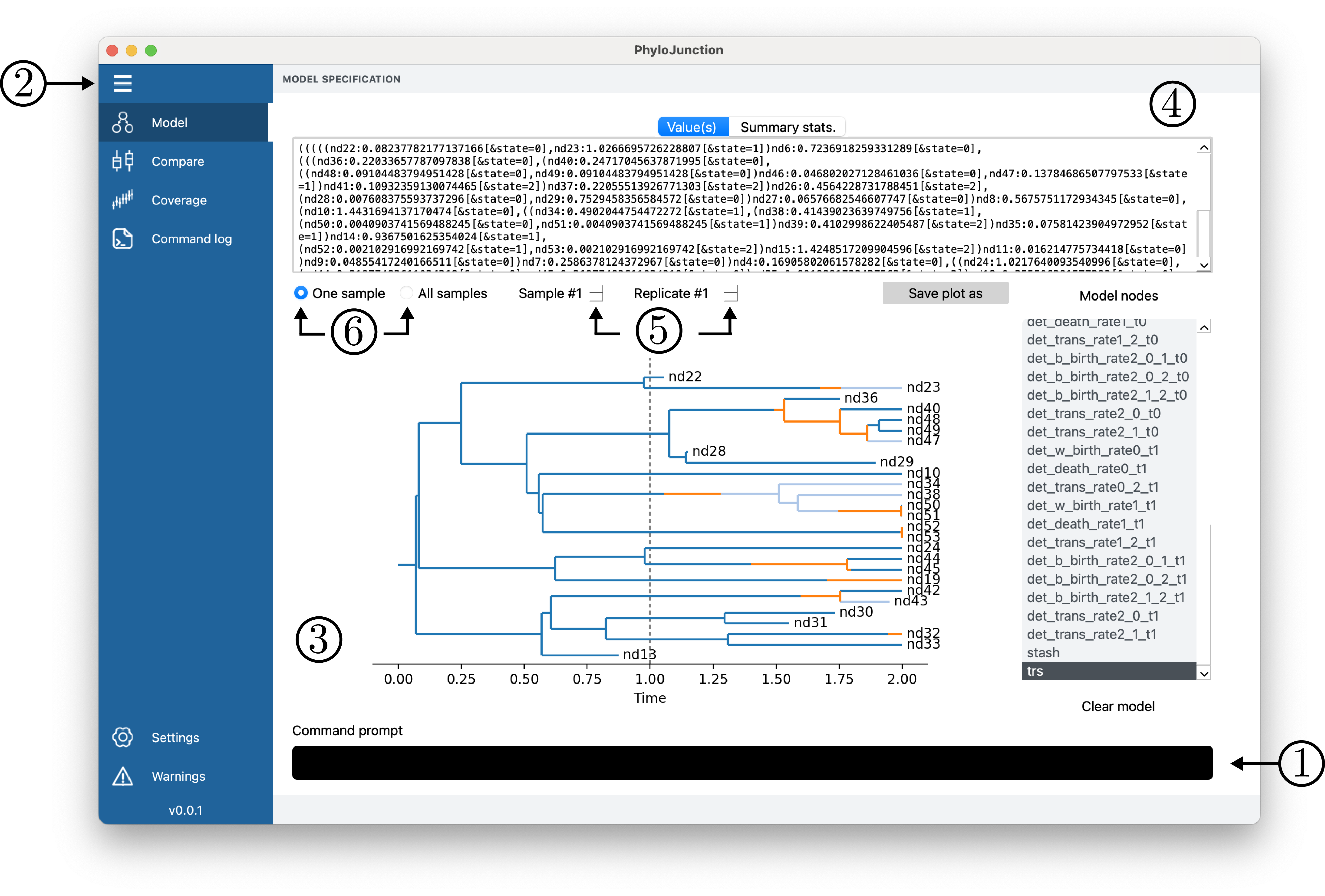
Figure 3. PhyloJunction’s GUI main window.
Like any modern computer application, PhyloJunction’s GUI exposes its features to users via a menu (Fig. 3, number 2). On the main tab (“Model”), one can build a model (DAG) with commands entered in the prompt (Fig. 3, number 1), or by loading a phylojunction script or a model from a previous PhyloJunction section. The latter can be done by clicking the application’s menu (top-left corner of the Desktop on Apple machines), and clicking “File > Read script” or “File > Load model”. Model building commands can be revisited by going into the menu’s “Command log” tab.
Warning
If mistakes are made when entering a command, PhyloJunction will flash a “Warning produced” message in red, at the bottom of the main window. The warning message can be seen by visiting the “Warnings” tab.
Given a model, DAG node values can be navigated as a plot, text string, or both (Fig. 3, numbers 3 and 4). Users can cycle through replicated simulations (Fig. 3, number 5), and examine node-value summaries computed for individual simulations or across replicates (Fig. 3, number 6). Node-value summaries include the mean and standard deviation for scalar variables, and statistics like the root age and number of tips for phylogenetic trees.
After a model is specified, saving the main plot (from the “Model” tab) to disk can be done by clicking “Save plot as”. Simulated data tables, or the model itself, in turn, can be saved to disk by clicking the application menu (top menu), and clicking “File > Save data as” or “File > Save model as”.
Implementation comparison
The “Compare” tab (under “Model”) streamlines the comparison of PhyloJunction’s simulations with those from an external simulator, with respect to a summary statistic. There are two main moments when carrying out this type of comparison may be useful or required. The first is when a model is being first implemented in PhyloJunction, and there happens to exist an independent implementation elsewhere. This latter implementation can be used to provide a baseline expectation for PhyloJunction.
Beyond model development within the platform, the “Compare” tab was further designed to expedite activities related to teaching. Students in an evolutionary modeling course may be asked to code their own Yule model, for example, in whatever programming language. After Yule trees are obtained, all they need to do is collect summary statistics that are also monitored by PhyloJunction (e.g., the root age), and upload them into the “Compare” tab. PhyloJunction then automatically plots the two distributions (one from the student, one from PhyloJunction itself) side by side, revealing if implementations behave similarly.
In order to use the functionalities exposed by the “Compare” tab, first one must to build a model in PhyloJunction. We can start with the simple model in examples/multiple_scalar_tree_plated.pj. As the name suggests, this model has a few different scalar and tree random variables, some of them plated. We can load it by clicking “File > Read script” and selecting the aforementioned file. By navigating to the “Compare” tab, you will see that PhyloJunction has loaded the DAG nodes that could potentially be compared on the left-hand “Nodes to compare” menu.
In the “Compare” tab, now click “Compare to .csv (…)”. This button allows user to input a .csv file containing summary statistics computed from external simulations. We will choose file examples/compare_files/comparison_multiple_scalar_tree_plated_rv5.csv. Once the .csv file is loaded, PhyloJunction should display the contents of it in the top window.
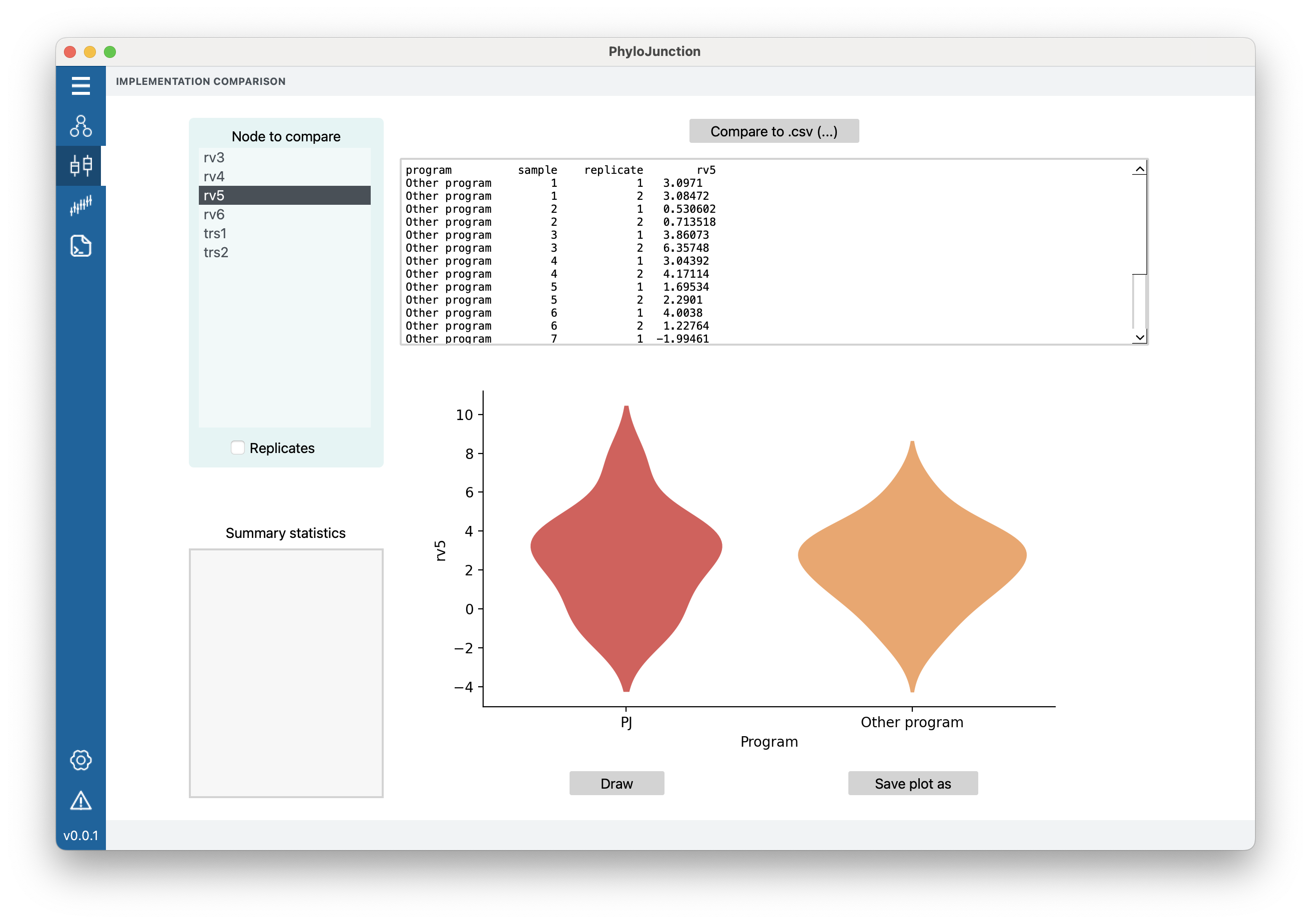
Figure 4. PhyloJunction’s GUI “Compare” tab.
Note the “rv5” column name at header of the table – these are the variable names that PhyloJunction will try to look up (and compare with) in its own model’s list of nodes. Accordingly, select “rv5” from the top-left “Node to compare” menu. Now we are ready to draw, click “Draw”. The produced graph (Fig. 4) should indicate that PhyloJunction and the external simulator behave similarly.
Let us now try a different random variable, a tree this time: click on node “trs2” on the “Node to compare” menu. Because tree space is complicated (there are both a discrete and a continuous dimensions to it, the topology and branch lengths, respectively), we will need to look at tree summary statistics. Different tree statistics should have been listed in the bottom-left “Summary statistics” menu. Choose one of them, “root age”, for example.
Now we must then load a different .csv file, examples/compare_files/comparison_multiple_scalar_tree_plated_trs2.csv. This file contains tree summary statistics presumably produced by a different external simulator. Click “Draw”. Again, the produced graph suggests the model implemented in both simulators behave similarly.
Coverage validation
The “Coverage” tab was developed for automating coverage validation, a procedure for verifying the correctness of a model implemented within a Bayesian framework. Coverage validation in fact validates multiple things simultaneously: the generating (simulator) and inferential implementations of the model, and any machinery used in inference (e.g., MCMC proposals). For the sake of clarity and conciseness, we will assume in this section that we are validating a model’s inferential engine, and that all other involved code works as intended.
The gist of coverage validation is straightforward: the \(\alpha\) %-HPD over a model parameter produced during Bayesian inference should contain the “true” (i.e., simulated) parameter value approximately \(\alpha\) % of the time. For example, if a stochastic node in the DAG is sampled 100 times (i.e., 100 i.i.d. random variables), then for approximately 95 of those simulations the 95%-HPD interval will contain the true sampled value.
In order to carry out coverage validation with the GUI, first we must build a model in PhyloJunction.
Click “File > Read script” and select examples/coverage_files/r_b_exp.pj.
In the loaded model, one hundred independent samples for a parameter \(r_b\) were assigned to a constant node r_b named after it.
These 100 values were drawn from an exponential distribution implemented elsewhere, but could also have been sampled directly in PhyloJunction.
In the “Coverage” tab, one can now load a .csv file containing a table with \(r_b\) ‘s posterior distribution’s mean value, and the lower and upper bounds of an HPD interval.
(This posterior distribution came from a Bayesian analysis done with a different program.)
The table headers must be posterior_mean, lower_95hpd, and higher_95hpd.
Click “Read HPDs .csv (…)”, and select examples/coverage_files/r_b_exp.csv.
The table should have been shown in the top middle window.
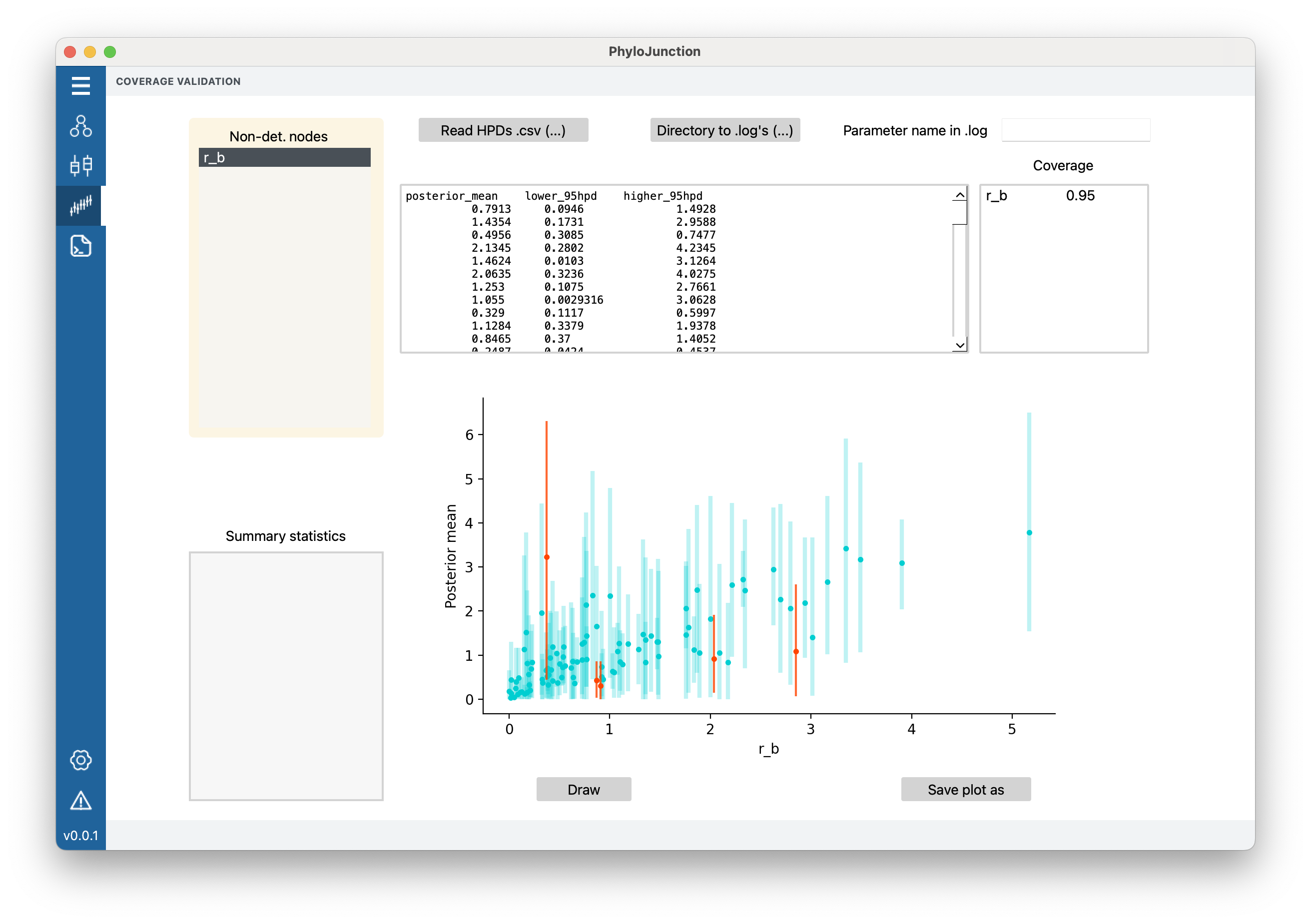
Figure 5. PhyloJunction’s GUI “Coverage” tab.
To inspect coverage, select “r_b” from the top-left menu “Non-det. nodes”, and then click on “Draw”. The x- and y-axes in the plot (the main panel in Fig. 5) show to the true simulated values and the posterior means, respectively. Vertical bars denote the 95%-HPDs over \(r_b\), with blue bars (95 of them) indicating intervals containing the true value, and red bars (5 of them) not containing it. In other words, one can deduce from the graph that coverage for \(r_b\) was 0.95 (though this is also shown in the top-right panel; Fig. 5); this coverage is adequate and indicative of a correctly implemented model.
In addition to loading a .csv file with pre-calculated posterior distribution summaries, users can also tell PhyloJunction the path of a directory containing MCMC output .log files. After loading the same model as before and clicking on “r_b” in the top-left menu, click on “Directory to .log’s (…)”, and choose examples/coverage_files/logfiles/. If in the .log files the node being examined were to be named something different from “r_b”, users can tell PhyloJunction what to look for by entering the alternative name in “Parameter name in .log”. For example, one could type “r_b” in “Parameter name in .log” (in this case it is not necessary).
Now click on “Draw”. An almost identical plot should have been produced, and coverage is again appropriate (0.94). (The difference of 1 in coverage has to do with the behavior of different libraries when computing HPD boundaries.)
Command-line interface (CLI)
PhyloJunction has a command-line interface (CLI) as an entry point for some of its functionalities – it is particularly handy when running PhyloJunction is a step in a longer pipeline (perhaps being run on a cluster).
The easiest way to see what is possible with the CLI is to call it on the Terminal with the -h flag, like so:
pjcli -h
The help message should list a series of flags, which we expand on below:
-d: Simulated data tables are written to disk.-f: Plots for the selected DAG nodes (whose names and sample ranges are passed as arguments) are written to disk. The argument for-fshould be passed within single-quotes, e.g., ‘birth_rate,trs;1-2,1-10’.-o: Directory where to place simulated data tables and figures.-p: Prefix to prepend output files with (e.g., “simulation1”)-nex: Certain simulated data is written to disk in NEXUS format.-r: Random seed so that simulations always produce the same output.
Note that if no argument is passed to -o, data tables written to disk (prompted by -d) will be placed in the directory from which PhyloJunction is called.
Figures (prompted by -f), in turn, will be placed in a “figures/” sub-directory, next to the data tables.
Sandbox: Bypassing the interfaces
Users and developers who wish to bypass PhyloJunction’s standalone interfaces to explore the code base can do so by using pj_sandbox.py.
Of course, some familiarity with Python is required.
The pj_sandbox.py script contains a few examples of how PhyloJunction can be imported as a module and used for different purposes.
Each example is wrapped within its own function, like so:
# pj imports
import phylojunction.interface.cmdbox.cmd_parse as cmdp
import phylojunction.pgm.pgm as pgm
...

def run_example_yule_string() -> pgm.DirectedAcyclicGraph:
    """Run example 1.

    This example sets up a simple Yule model with two samples,
    and two Yule tree replicates per sample.
    """

    yule_model_str = \
        ('n_sim <- 2\nn_rep <- 2\nbirth_rate <- 1.0\n'
         'det_birth_rate := sse_rate(name="lambda", value=birth_rate,'
         ' event="speciation")\n'
         'stash := sse_stash(flat_rate_mat=[det_birth_rate])\n'
         'trs ~ discrete_sse(n=n_sim, nr=n_rep, stash=stash, start_state=[0],'
         ' stop="size", stop_value=10.0, origin="false")\n')

    dag_obj = cmdp.script2dag(yule_model_str, in_pj_file=False)

    return dag_obj
The example above is then invoked later in pj_sandbox.py:
Calling example 1 in pj_sandbox.py. Which example to execute can be specified in the script main body.dag_obj: pgm.DirectedAcyclicGraph = pgm.DirectedAcyclicGraph() ... # examples # 1: Yule model string, 2 tree samples, 2 tree replicates per sample # 2: Same as (1), but reading a pre-made .pj script in examples/yule.pj # 3: BiSSE model with incomplete sample, 2 tree samples, 2 tree replicates per sample # 4: Builds discrete SSE tree manually, then prints on screen # 5: Builds discrete SSE tree from newick string, then prints on screen # 6: Read .pj script examples/see_stoch_maps.pj example_to_run = 1 # example_to_run = 2 # example_to_run = 3 # example_to_run = 4 # example_to_run = 5 # example_to_run = 6 if example_to_run == 1: dag_obj = run_example_yule_string() ...
Lexicon
Parametric distributions
PhyloJunction ships with a (growing) number of parametric distributions. All distributions support replication (i.e., plating in the DAG) and take as arguments both direct scalar values (e.g., “1.0”) and values stored in DAG nodes. On this page you will find examples of how to invoke the available distributions (using the phylojunction language) when building a model.
Uniform
The function for assigning a uniform (uniform) distribution to a random variable has four parameters:
n(integer, optional): Number of samples to draw (samples are i.i.d.). Defaults to 1.nr(integer, optional): Number of replicates to draw per sample. Defaults to 1.min(real number, required): Lower bound (inclusive).max(real number, required): Upper bound (inclusive).
x ~ unif(n=2, nr=2, min=-1.0, max=1.0)
Exponential
The function for assigning a exponential (exponential) distribution to a random variable has four parameters:
n(integer, optional): Number of samples to draw (samples are i.i.d.). Defaults to 1.nr(integer, optional): Number of replicates to draw per sample. Defaults to 1.rate(positive real, required): Rate (or scale) of distribution.rate_parameterization(string boolean, optional): Whether the value passed inrateis the distribution’s rate. Defaults to “true”.
x ~ exponential(n=2, nr=2, rate=1.0, rate_parameterization="false")
Gamma
The function for assigning a gamma (gamma) distribution to a random variable has five parameters:
n(integer, optional): Number of samples to draw (samples are i.i.d.). Defaults to 1.nr(integer, optional): Number of replicates to draw per sample. Defaults to 1.shape(positive real, required): Shape of distribution.scale(positive real, required): Scale (or rate) of distribution.rate_parameterization(string boolean, optional): Whether the value passed inscaleis the distribution’s rate. Defaults to “false”.
x ~ gamma(n=2, nr=2, shape=10.0, scale=1.0)
Normal
The function for assigning a normal (normal) distribution to a random variable has four parameters:
n(integer, optional): Number of samples to draw (samples are i.i.d.). Defaults to 1.nr(integer, optional): Number of replicates to draw per sample. Defaults to 1.mean(real, required): Mean (location) of distribution.sd(positive real, required): Standard deviation (scale) of distribution.
x ~ normal(n=2, nr=2, mean=0.0, sd=1.0)
Log-normal
The function for assigning a log-normal (lognormal) distribution to a random variable has five parameters:
n(integer, optional): Number of samples to draw (samples are i.i.d.). Defaults to 1.nr(integer, optional): Number of replicates to draw per sample. Defaults to 1.meanlog(real, required): Mean (location) of distribution over the logarithm of the random variable.sdlog(positive real, required): Standard deviation (scale) of distribution over the logarithm of the random variable.log_space(string boolean, optional): Whether the value ofmeanis in log-space. Defaults to “true”.
x ~ lognormal(n=1000, mean=-3.25, sd=0.25)
Categorical
The function for assigning a categorical (categorical) distribution to a random variable has four parameters:
n(integer, optional): Number of samples to draw (samples are i.i.d.). Defaults to 1.nr(integer, optional): Number of replicates to draw per sample. Defaults to 1.cats(integer, required): Number of discrete categories in each draw (must be greater than 1).probs(real number, required): Probability of each category (must add up to 1.0).
x ~ categorical(n=2, nr=2, cats=[0,1], probs=[0.5, 0.5])
Tree distributions
Phylogenetic tree stochastic nodes can be added to a model’s DAG using tree distributions. At the moment, PhyloJunction comes with one tree distribution that produce a variety of tree types.
Discrete SSE
Discrete SSE (discrete_sse) stands for discrete state-dependent speciation and extinction process, a general model that includes many popular special cases documented below.
Rate types
The implementation and usage of discrete_sse in PhyloJunction is very flexible and takes inspiration from Tim Vaughan’s great ReMASTER simulator program: a model with any number of rates of whatever types may be specified.
Of course, this flexibility comes at the price of user responsibility!
SSE rates are added to a DAG by passing deterministic function sse_rate a stochastic or constant node containing a rate’s value (the value can also be passed directly):
birth_rate ~ exponential(n=2, nr=2, rate=1.0)

det_birth_rate := sse_rate(name="lambda", value=birth_rate, event="speciation")

# alternatively, one could pass values directly to sse_rate()
# det_birth_rate := sse_rate(name="lambda", value=[0.95, 1.05], event="speciation")
Parameters for sse_rate include:
name(string, required): The name of the rate parameter. Not particularly critical other than for printing sensical messages to the screen, when using the GUI. The argument tonamedoes not have to match anything else in the model, and can in practice be any string enclosed in double quotes.value(positive real, required): The rate value. This parameter can also take the name of other nodes in the DAG (in which case the value of those nodes are extracted and used).event(string, required): A string specifying the rate type (see below).epoch(positive integer, optional): Integer specifying the epoch to which this rate applies. See more in the “Time-heterogeneity” section below. Defaults to 1.Arguments for theeventparameter should be enclosed in double quotes and can be:
"speciation"or"w_speciation"for within-state birth rates;
"b_speciation"for between-state birth rates;
"asym_speciation"for asymmetric birth rates;
"extinction"for extinction rates;
"transition"for anagenetic transition rates;
"anc_sampling"for ancestor sampling (e.g., “fossilization”) rates.
Sampling probabilities
The discrete SSE model in PhyloJunction supports not only state-dependent rates, but also state-dependent sampling probabilities. Specifying SSE probabilities can be done like so:
det_sampling_prob := sse_prob(name="rho", value=1.0, state=0)
# by setting the value to 1.0, we assume complete sampling!
The parameters for sse_prob are:
name(string, required): The name of the probability parameter. Behaves the same as the name of SSE rate parameters.value(real between 0.0 and 1.0, required): The probability value. As with SSE rates, this parameter can also take the name of DAG nodes that hold probability values.state(positive integer starting at 0, optional): This integer represents the state to which the probability is associated. Defaults to 0.epoch(positive integer, optional): Integer specifying the epoch to which this probability applies. See more in the “Time-heterogeneity” section below. Defaults to 1.
Note that the state parameter defaults to 0, and is the state value used in non-state-dependent tree models, like the Yule or birth-death models.
The SSE stash (and time-heterogeneity)
Before discrete_sse can be assigned as the tree distribution to a DAG stochastic node, state-dependent rate and probability parameters must be stashed together and combined with some more information.
This is accomplished with deterministic function sse_stash, whose parameters are:
flat_rate_mat(string vector, required): A vector (deterministic) DAG node names holding the objects created withsse_rate. DAG node names do not have to appear in any specific order.flat_prob_mat(string vector, required): A vector (deterministic) DAG node names holding the objects created withsse_prob. DAG node names do not have to appear in any specific order.n_states(positive integer, optional): How many states the SSE process has. Defaults to 1.n_epochs(positive integer, optional): How many epochs characterize the skyline of the SSE process. Defaults to 1.seed_age(positive real, optional): The age of the node at which the SSE process starts (either the origin or root node). This parameter must receive an argument if parameters are time-heterogeneous, and it must match the value given tostop_valuewhen specifyingdiscrete_ssewithstop="age"(see more below).epoch_age_ends(positive real vector, optional): The age of the ends of each epoch (i.e., the “younger” limit of each epoch, measured as an age), going from the oldest to the youngest epoch. The end of the youngest epoch (which contains the present) should be ommitted as it is added by default. The number of provided age ends should thus be the number of epochs (inn_epochs) minus one. Defaults to [0.0].
The discrete SSE model in PhyloJunction is a “skyline” model, that is, it allows both state-dependent rates and parameters to vary over time (i.e., to be time-heterogeneous).
In the presence of time-heterogeneity, these parameters are assumed to vary according to a user-defined piecewise constant function (this is coded into the model via the value and epoch parameters of sse_rate and sse_prob).
The limits of each “piece” of that function are given by the argument to epoch_age_ends (see above).
det_birth_rate1 := sse_rate(name="lambda1", value=1.0, event="speciation", epoch=1)
det_birth_rate2 := sse_rate(name="lambda2", value=2.0, event="speciation", epoch=2)

stash := sse_stash(flat_rate_mat=[det_birth_rate1, det_birth_rate2], n_epochs=2, seed_age=2.0, epoch_age_ends=[1.0])
# there are two epochs, the oldest one ends at age 1.0, the youngest one ends at the present
# the birth-rate of the oldest epoch is 1.0, but that rate doubles in the youngest epoch
The discrete SSE distribution
We have seen how to add to the DAG a series of ingredients required by the discrete_sse distribution.
The parameters of this function are:
n(integer, optional): Number of samples to draw (samples are i.i.d.). Defaults to 1.nr(integer, optional): Number of replicates to draw per sample. Defaults to 1.stash(string, required): Name of DAG node holding the object created bysse_stash.start_state(positive integer vector starting at 0, required): State at which the process starts for each sample.stop(string, required): String specifying the simulation stopping condition. If set to"age", the simulation will stop when the origin or root’s age (see parameterorigin) reaches the value provided instop_value. If set to"size", the simulation will stop when the tree has the number of sampled nodes provided instop_value.stop_value(positive numeric, required): The stopping condition threshold. Ifstop="age", this can be any positive real number. Ifstop="size", this can be any positive integer.origin(string boolean, required): Flag specifying if process starts at origin node (as opposed to the root node). Defaults to “true”.cond_spn(string boolean, optional): Condition the process on at least one speciation event happening. Note that this speciation event may or not be the event represented by the root of the reconstructed tree. Defaults to “false”.cond_surv(string boolean, optional): Condition the process on having at least one surviving lineage at the present moment. This conditioning only makes sense whenstop="age". Defaults to “true”.cond_obs_both_sides(string boolean, optional): Condition the process on having sampled nodes on both sides of the complete tree’s root node. Defaults to “false”.min_rec_taxa(positive integer, optional): Minimum number of sampled (extant and sampled ancestors) nodes the tree should have. Defaults to 0.max_rec_taxa(positive integer, optional): Maximum number of sampled (extant and sampled ancestors) nodes the tree should have. Defaults to 1e12.abort_at_alive_count(positive integer, optional): The count of a tree’s living nodes (irrespective of node sampling) at which point the tree is considered too large for simulation to continue. Trees can grow out of control whenstop="age"and one of the rates allows it to grow too big before the stopping condition is met. This parameter can be used to throw away such trees and preventing PhyloJunction from crashing. Defaults to 1e12.runtime_limit(positive integer, optional): Maximum number of seconds to wait until all samples are drawn. Sampling is aborted at this point. Defaults to 300.max_n_attempts(positive integer, optional): Maximum number of (failed) attempts before sampling is aborted. Defaults to 200.
Below, an example of assigning a discrete SSE to a stochastic DAG node representing phylogenetic tree samples:
det_birth_rate1 := sse_rate(name="lambda1", value=1.0, event="speciation", epoch=1)
det_birth_rate2 := sse_rate(name="lambda2", value=2.0, event="speciation", epoch=2)

stash := sse_stash(flat_rate_mat=[det_birth_rate1, det_birth_rate2], n_epochs=2, seed_age=2.0, epoch_age_ends=[1.0])

trs ~ discrete_sse(n=2, stash=stash, start_state=[0,0], stop="age", stop_value=2.0, origin="true")
Special cases of discrete SSE tree models
Yule (pure-birth) model;
Birth-death model;
Fossilized birth-death (FBD) model;
Binary state-dependent speciation and extinction (BiSSE) model;
Time-heterogeneous binary state-dependent speciation and extinction (skyline BiSSE) model;
Geographic state-dependent speciation and extinction (GeoSSE) model;
Time-heterogeneous geographic state-dependent speciation and extinction (skyline GeoSSE) model;